Have you ever wondered how to create a stacked column chart percentage in Excel? Well, you’re in luck! This handy guide will walk you through the steps to make your data come to life visually.
Creating a stacked column chart percentage is a great way to showcase your data in a clear and concise manner. Whether you’re a student working on a project or a professional presenting to your team, this chart type can help you communicate your message effectively.

Stacked Column Chart Percentage
Stacked Column Chart Percentage: Step-by-Step Guide
To begin, open Excel and input your data into a spreadsheet. Make sure to include all the necessary columns and rows for your chart. Next, select the data you want to include in your stacked column chart percentage.
Once you have selected your data, navigate to the “Insert” tab on the Excel toolbar. From there, choose the “Column” chart option and then select the stacked column chart type. This will automatically generate a basic stacked column chart for you.
Now it’s time to customize your chart to display percentages. Right-click on the chart and select “Format Data Series.” From there, navigate to the “Series Options” tab and choose the option to display percentages. Voila! Your stacked column chart now shows percentages.
In conclusion, creating a stacked column chart percentage in Excel is a simple and effective way to visualize your data. By following these easy steps, you can impress your audience and communicate your message clearly. Give it a try and see the difference it makes in your presentations!