Have you ever wanted to create a visually appealing stacked column chart from a pivot table in Excel? With just a few simple steps, you can easily showcase your data in a way that is both informative and visually appealing.
By utilizing the pivot table feature in Excel, you can organize and summarize your data quickly and efficiently. Once you have your pivot table set up with the desired data fields, creating a stacked column chart is a breeze.
Stacked Column Chart From Pivot Table
Stacked Column Chart From Pivot Table
To create a stacked column chart from your pivot table data, simply select the cells containing the data you want to visualize, then navigate to the “Insert” tab and choose the “Column Chart” option. From there, select the “Stacked Column” chart type.
Customize your chart by adding data labels, changing colors, and adjusting the axis titles to make it more visually appealing. You can also easily update your chart as your pivot table data changes, ensuring that your visualizations are always up to date.
With a stacked column chart from a pivot table, you can easily see how different data points contribute to the overall total. This visual representation can help you identify trends, patterns, and outliers in your data at a glance.
Next time you need to present data in a clear and concise manner, consider creating a stacked column chart from your pivot table in Excel. It’s a simple yet powerful way to showcase your data and make informed decisions based on the insights gained.