Are you looking to learn how to hide a column from a pivot table chart? Look no further! With just a few simple steps, you can easily customize your pivot table chart to show only the data you want.
When working with pivot tables in Excel, sometimes you may want to hide certain columns from your chart to focus on specific data points. This can be useful for creating a cleaner and more organized visualization of your data.

Pivot Table Hide Column From Chart
Pivot Table Hide Column From Chart
To hide a column from a pivot table chart, first, select the column you want to hide. Then, right-click on the column header and choose “Hide” from the drop-down menu. The column will be hidden from the chart while still being available in the pivot table.
Alternatively, you can also hide a column by selecting the column header and pressing “Ctrl” + “-” on your keyboard. This keyboard shortcut will hide the selected column from the chart instantly.
Remember that hiding a column from a pivot table chart does not delete the data; it simply removes it from the visual representation. You can always unhide the column by right-clicking on the pivot table and selecting “Unhide” or by pressing “Ctrl” + “+” on your keyboard.
By following these simple steps, you can easily customize your pivot table chart to display only the data that is most relevant to your analysis. So go ahead and give it a try next time you’re working with pivot tables in Excel!