Have you ever wanted to create a pivot chart in Excel but only include data from specific columns? Well, you’re in luck! With a few simple steps, you can easily customize your pivot chart to display only the information you need.
When working with a large dataset in Excel, it can be overwhelming to create a pivot chart that includes every single column. By using the “PivotChart Only Some Columns” feature, you can focus on the most relevant data and make your chart more visually appealing.

Pivot Chart Only Some Columns
Pivot Chart Only Some Columns
To start customizing your pivot chart, simply select the columns you want to include by checking or unchecking the boxes next to each column in the PivotChart Fields pane. This allows you to tailor your chart to display only the information that is important to you.
By narrowing down the columns in your pivot chart, you can easily spot trends, patterns, and outliers in your data. This targeted approach not only makes your chart more visually appealing but also helps you analyze the data more effectively.
Don’t forget to experiment with different column combinations to see which ones provide the most valuable insights. You can always go back and adjust the columns in your pivot chart to refine your analysis and make informed decisions based on the data.
With the “PivotChart Only Some Columns” feature in Excel, you have the flexibility to create customized pivot charts that showcase the most relevant data for your analysis. So why wait? Start exploring this powerful tool today and take your data visualization skills to the next level!