If you’ve ever struggled with linking two chart columns headers together, you’re not alone. This common issue can be frustrating, but with a few simple steps, you can easily overcome it.
Many people find themselves in a situation where they have multiple columns in a chart and want to link the headers of two specific columns together. This can be useful for creating dynamic charts that update automatically based on your data.

Link Two Chart Columns Headers Together
Link Two Chart Columns Headers Together
One way to achieve this is by using Excel’s built-in feature called data validation. By setting up a drop-down list in one column that is dependent on the selection in another column, you can effectively link the two headers together.
Start by selecting the cells where you want the drop-down lists to appear. Then, go to the Data tab, click on Data Validation, and choose List as the validation criteria. In the Source box, enter the range of values you want to appear in the drop-down list.
Once you have set up the data validation for both columns, you will see that the headers are now linked together. When you select a value in one column, the corresponding values in the other column will automatically update based on your selection.
By following these simple steps, you can easily link two chart columns headers together in Excel. This can help you create more dynamic and interactive charts that make it easier to analyze and visualize your data.
Next time you find yourself struggling with linking headers in your Excel charts, remember these tips and make your data analysis process a breeze.

Format Your Page Notion Help Center