Have you ever wanted to change the orientation of your column chart in Excel? By inverting the column chart axis, you can easily display your data in a different way. In this article, we’ll show you how to do just that!
When you invert the axis of your column chart, the values are displayed in reverse order. This can be useful when you want to emphasize the highest or lowest values in your data set. It’s a simple but effective way to make your charts more impactful.

Inverting Your Column Chart Axis
Inverting Your Column Chart Axis
To invert the axis of your column chart in Excel, simply right-click on the axis you want to invert. Then, select “Format Axis” from the dropdown menu. In the Format Axis pane, check the box next to “Values in reverse order.” That’s it!
By inverting the axis of your column chart, you can create a more visually appealing representation of your data. This can help you better understand trends and patterns in your data, making it easier to draw insights and make informed decisions.
Experiment with inverting the axis of your column charts in Excel to see how it can enhance the visual impact of your data. Whether you’re creating a chart for a presentation, report, or just for fun, this simple technique can take your data visualization to the next level.
So go ahead and give it a try! Inverting the axis of your column chart in Excel is a quick and easy way to make your data stand out. You’ll be amazed at how such a small change can make a big difference in the way your data is presented.