If you’re looking to enhance your data visualization skills in Excel, learning how to insert a clustered column pivot chart is a great place to start. This type of chart can help you easily compare data across different categories.
By inserting a clustered column pivot chart, you can quickly see trends and patterns in your data, making it easier to make informed decisions. Whether you’re a business professional, student, or data enthusiast, mastering this skill can be incredibly beneficial.

Insert A Clustered Column Pivot Chart
Insert A Clustered Column Pivot Chart
To insert a clustered column pivot chart in Excel, start by selecting the data you want to include in the chart. Then, go to the Insert tab, click on PivotChart, and choose the clustered column chart option. From there, you can customize the chart to suit your needs.
One of the advantages of using a clustered column pivot chart is that it allows you to compare multiple data series side by side. This can help you identify correlations, outliers, and other important insights that may not be immediately apparent when looking at raw data.
Whether you’re analyzing sales figures, survey responses, or any other type of data, a clustered column pivot chart can help you visualize the information in a clear and concise manner. With a little practice, you’ll be able to create professional-looking charts that effectively communicate your findings.
So, next time you’re working with data in Excel, consider inserting a clustered column pivot chart to take your analysis to the next level. It’s a simple yet powerful tool that can make a big difference in how you interpret and present your data.