Are you tired of endless scrolling through rows of data in your pivot chart? Do you wish there was an easier way to see the big picture at a glance? Well, you’re in luck! By including a total column in your pivot chart, you can simplify your data analysis and make informed decisions faster.
Adding a total column to your pivot chart allows you to quickly see the sum, average, count, or other aggregate functions of your data. This can help you identify trends, outliers, and patterns that may not be immediately apparent when looking at individual data points.

Include Total Column In Pivot Chart
Include Total Column In Pivot Chart
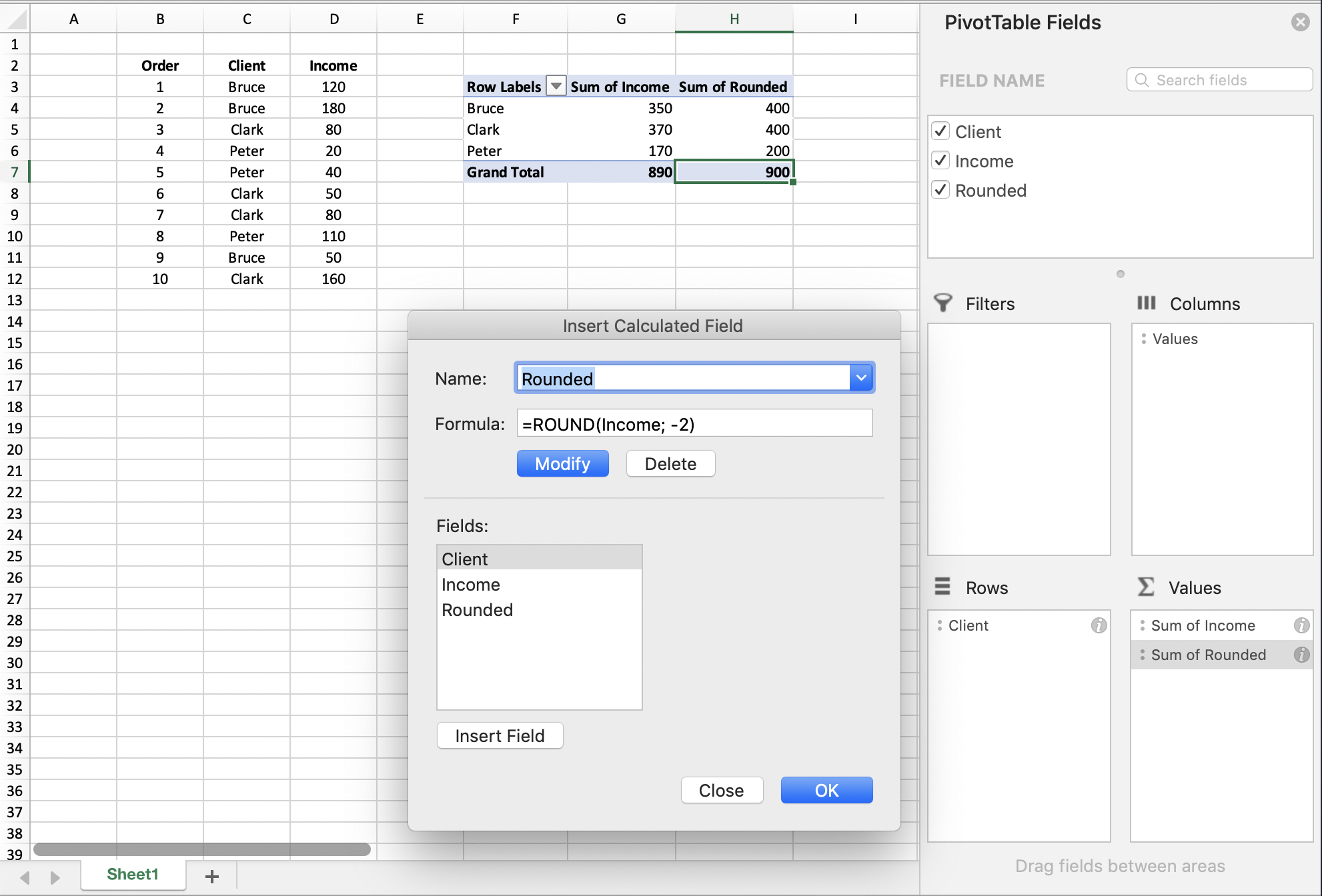
To add a total column to your pivot chart, simply click on the “Design” tab in Excel, then select “Grand Totals” and choose where you want the totals to be displayed – either at the bottom or top of your chart. Voila! You now have a total column that provides a comprehensive overview of your data.
With a total column in your pivot chart, you can easily compare different categories, track progress over time, and make data-driven decisions with confidence. Say goodbye to manual calculations and hello to a more efficient and effective way of analyzing your data.
So, next time you’re working with a pivot chart in Excel, don’t forget to include a total column for a clearer and more comprehensive view of your data. Your future self will thank you for making data analysis a breeze!