Are you tired of spending hours creating clustered column charts in Excel? Well, we’ve got a shortcut that will save you time and frustration. In just a few simple steps, you can create professional-looking charts in no time!
With the Clustered Column Chart Shortcut, you can easily visualize your data and make informed decisions. Whether you’re a student working on a project or a professional analyzing business trends, this shortcut will be your new best friend.
Clustered Column Chart Shortcut
Creating a Clustered Column Chart Shortcut
To start, select the data you want to include in your chart. Then, go to the “Insert” tab on the Excel ribbon and click on the “Column” chart icon. From the dropdown menu, choose the “Clustered Column” option.
Next, customize your chart by adding titles, labels, and adjusting the colors to suit your preferences. You can also easily switch between different chart styles to find the one that best represents your data.
Once you’re satisfied with your clustered column chart, you can easily copy and paste it into your presentations, reports, or share it with colleagues. With this shortcut, you’ll impress everyone with your data visualization skills!
So, next time you need to create a clustered column chart in Excel, remember this simple shortcut. It will not only save you time but also help you create professional-looking charts with ease. Give it a try and see the difference it makes in your data analysis!