Are you looking to create visually appealing and informative pivot charts in Excel? One useful tool you can utilize is the Cluster Column Pivot Chart. This feature allows you to display your data in a clear and organized manner.
With a Cluster Column Pivot Chart, you can easily compare data across different categories. This type of chart is perfect for showcasing trends, patterns, and comparisons within your dataset. It’s a great way to present your information in a visually engaging format.
Cluster Column Pivot Chart
Creating a Cluster Column Pivot Chart
To create a Cluster Column Pivot Chart in Excel, start by selecting your data range. Then, go to the Insert tab and choose PivotChart. From the PivotChart Fields pane, drag and drop the fields you want to display into the Axis and Values areas. Finally, select Clustered Column as the chart type.
Once you have your Cluster Column Pivot Chart set up, you can customize it further by adding titles, labels, and formatting options. This allows you to tailor the chart to suit your specific needs and preferences. Experiment with different settings to find the best layout for your data.
Cluster Column Pivot Charts are a powerful tool for analyzing and presenting data in Excel. Whether you’re working on a business report, project analysis, or any other data-driven task, these charts can help you convey your findings effectively. Try using Cluster Column Pivot Charts in your next Excel project and see the difference they can make!
In conclusion, Cluster Column Pivot Charts are a versatile and user-friendly feature that can enhance your data visualization in Excel. By utilizing these charts, you can create dynamic and compelling representations of your data that are easy to understand and interpret. Give them a try and take your Excel skills to the next level!