Are you looking to easily chart aggregate data in Column A of your spreadsheet? Look no further! With these simple steps, you’ll be able to visualize your data in no time.
First, select the range of data in Column A that you want to include in your chart. This could be anything from sales figures to survey responses, the choice is yours!

Chart Aggregate Column A
Chart Aggregate Column A
Next, navigate to the “Insert” tab on your spreadsheet software and choose the type of chart you want to create. Whether it’s a bar chart, pie chart, or line graph, make sure it best represents your data.
Once you’ve selected your chart type, customize it to your liking. Add titles, labels, and colors that make your data pop. Don’t be afraid to experiment until you find the perfect visual representation.
Finally, sit back and admire your work! Your chart should now be displaying the aggregate data from Column A in a clear and concise manner. Feel free to share it with colleagues or use it in your next presentation.
Now that you’ve mastered charting aggregate data in Column A, you can apply these same techniques to other columns in your spreadsheet. Get creative with your data visualization and unlock new insights with the power of charts!