Have you ever wondered how to create a 2 way column chart in Excel? Well, you’re in luck! In this article, we’ll walk you through the steps to make a visually appealing and informative chart that will impress your colleagues and boss.
Whether you’re a data analyst, business owner, or student, knowing how to create a 2 way column chart can be a valuable skill. It allows you to compare two sets of data in a clear and concise way, making it easier to identify trends and patterns.

2 Way Column Chart
Creating a 2 Way Column Chart
To create a 2 way column chart in Excel, start by selecting your data sets. Go to the “Insert” tab, click on “Column Chart,” and choose the 2D Clustered Column Chart option. Next, input your data into the spreadsheet and watch as Excel generates the chart for you.
You can customize your 2 way column chart by adding titles, labels, and legends to make it more visually appealing. You can also change the colors and styles of the columns to match your preferences or company branding.
Once you’ve created your 2 way column chart, take the time to analyze the data and draw insights from it. Look for trends, patterns, or anomalies that can help you make informed decisions and drive business growth. Share your findings with your team to collaborate and brainstorm ideas.
In conclusion, creating a 2 way column chart in Excel is a simple yet powerful way to visualize and analyze data. Whether you’re presenting to clients, stakeholders, or colleagues, a well-crafted chart can help you convey your message effectively and make data-driven decisions. So next time you have data to analyze, consider using a 2 way column chart to make your information more engaging and impactful.